Bayesian Modeling and Prediction for Movies
Description
This is my final project for a Bayesian Statistics course from Coursera. I had to create a bayesian predictive regression model that would predict the audience score of a movie given a host of review metrics.
Setup
Load packages
library(ggplot2)
library(dplyr)
library(statsr)
library(BAS)
library(GGally)
library(gridExtra)
Load data
load("C:/Users/aknorr/Desktop/movie_data.Rdata")Part 1: Data
The data for this predictive model on movie popularity were gathered from two main sources; IMDB and Rotten Tomatoes (RT). The movies contained in the data set were collected as a random sample and represent 651 titles released before 2016. Due to the nature of the data collect (random sampling) I feel confident that the titles included in this analysis are representative of the general population of movies. This means that our predictive model is generalizable to the larger population, and will be a good estimate of movie popularity. Though it is generalizable, this study will not be causal. There is selection bias in the data due to the types of people reviewing the movies. Critics and submissions from IMDB/ RT are not randomly assigned. It is people who either have a job to review movies, or have seen the movie and had a strong enough opinion to post it on one of these review sites. With that in mind we cannot confidently say the coefficicents have a causal impact on why the movie is popular or not. In addition, our dependent variable is based off those who go see the movie, and the group who selects into this treatment is not random (for all the same reasons that critics/ reviews are not random).
Part 2: Data manipulation
#Feature Film Var
movies$feature_film <- factor(rep(NA, length(movies$title_type)), levels = c("Yes", "No"))

movies$feature_film[movies$title_type == "Feature Film"] <- "Yes"
movies$feature_film[movies$title_type != "Feature Film"] <- "No"

#Drama
movies$drama <- factor(rep(NA, length(movies$genre)), levels = c("Yes", "No"))

movies$drama[movies$genre == "Drama"] <- "Yes"
movies$drama[movies$genre != "Drama"] <- "No"

#R Rating
movies$mpaa_rating_R <- factor(rep(NA, length(movies$mpaa_rating)), levels = c("Yes", "No"))

movies$mpaa_rating_R[movies$mpaa_rating == "R"] <- "Yes"
movies$mpaa_rating_R[movies$mpaa_rating != "R"] <- "No"

##Oscar
movies$oscar_season <- factor(rep(NA, length(movies$thtr_rel_month)), levels = c("Yes", "No"))

movies$oscar_season[movies$thtr_rel_month %in% c(10,11,12) ] <- "Yes"
movies$oscar_season[is.na(movies$oscar_season)] <- "No"

##Summer
movies$summer_season <- factor(rep(NA, length(movies$thtr_rel_month)), levels = c("Yes", "No"))

movies$summer_season[movies$thtr_rel_month %in% c(5,6,7,8) ] <- "Yes"
movies$summer_season[is.na(movies$summer_season)] <- "No"
Part 3: Exploratory data analysis
Table 3.1 Audience Score Summary Statistics
| audience_score | |
|---|---|
| Min. :11.00 | |
| 1st Qu.:46.00 | |
| Median :65.00 | |
| Mean :62.36 | |
| 3rd Qu.:80.00 | |
| Max. :97.00 |
Table 3.1 presents the summary statistics for audience scores recorded in the data set. These scores are based on user reviews from RottenTomateoes.com and Flixster.com and are scored from 0 to 100. The data has a strong left skew with a median score of 65 and a mean score of 62.36. The minimum score in the data set is 11 and the maximum score in the data set is 97. There are no movies which contain a missing value for audience score in the data set.
Figure 3.1 Audience Score and Feature Film Summaries
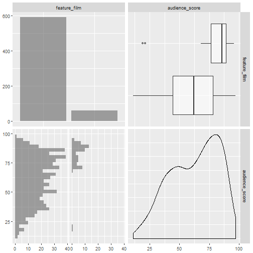
Figure 3.1 shows the relation of audience score and the first new variable, whether the movie is a feature film or not. The majority of the movies in the data set are feature films, 591 out of the 651 films. Audience scores seem to be normally distributed across the feature films with a mean of 60.47 and a median of 62. The remaining 60 films which are not considered feature films are not normally distributed. The mean is 81.05 and the median score is 85.5. The non-feature films also contain two outliers at extremely low audience scores (19, and 21).
Figure 3.2 Audience Score and Drama Summaries
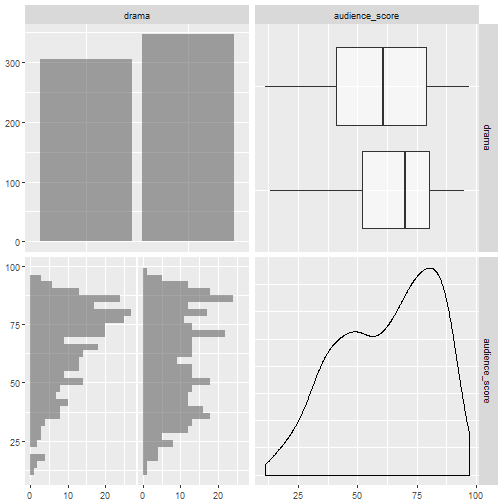
Figure 3.2 presents whether a film is a drama or not and the related audience scores. Splitting the data set by whether a film is a drama or not is fairly even; 305 Yes vs. 346 No. The films that are dramas have a slight left skew with a median of 70 and mean of 65.35. The films which are not considered dramas are normally distributed. There are no outliers.
Figure 3.3 Audience Score and R Rating Summaries
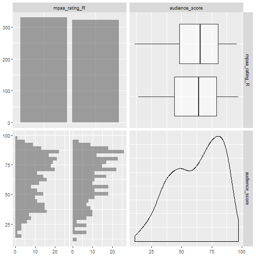
The data set is split fairly evenly between R rated, and non-R rated movies. Figure 3.3 shows that there are 329 R rated movies and 322 non-R rated movies. Both types of movies have similar distributions and similar means.
Figure 3.4 Audience Score and Oscar Season Summaries
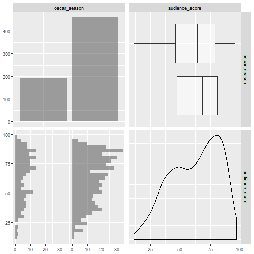
Figure 3.5 Audience Score and Summer Season Summaries
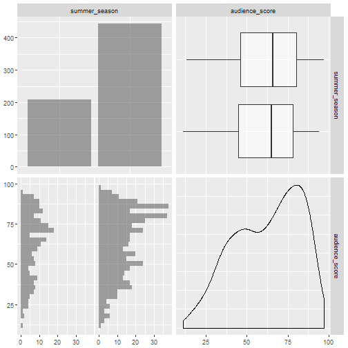
The final two figures examine oscar season and the summer time. Figure 3.4 and Figure 3.5 show that these groups both contain about 200 of all observations. And the distributions are similar across Yes or No for both oscar season and summer time. Finally, the means of audience score are about the same between summer time but the means of audience score are slightly different for oscar season (higher for those in oscar season).
Part 4: Modeling
movies_rm <- na.omit(movies)

bma_movies <- bas.lm(audience_score ~ feature_film + drama + runtime + mpaa_rating_R + thtr_rel_year + oscar_season + summer_season + imdb_rating + imdb_num_votes + critics_score + best_pic_nom + best_pic_win + best_actor_win + best_actress_win + best_dir_win + top200_box,
                     data = movies_rm,
                     prior = "ZS-null",
                     modelprior = uniform(),
                     method = "MCMC")

sum_model <- summary(bma_movies)
To build the predictive model I began with all the requested variables and used Bayesian Model Averaging (BMA) method to find the optimal model and optimal variables to include. Note, I have removed any observations which contained any NA values. These NA values were unsystematic and removal of rows with randomly distributed NAs is not a problem. This reduced my data set from 651 to 619. The prior is specified as Zellner Cauchy and the modelprior is set to a uniform dsitribution. Finally, I included MCMC so enumeration is not used. The optimal model included four coefficients; the intercept, the runtime, the IMDB rating, and the critics score (Figure 4.4). All four of these coeficients had an inclusion probability above .5. The optimal model had a BIC of -828.45 after transforming the presented logmarg of 414.2254. In addition to the BIC of -828.45, the optimal model had an R-squared of 74.55%. Figure 4.1 plots the residuals against the fitted values. Figure 4.2 shows the progression of cumulative probability and search order. Figure 4.3 identifies the optimal number of model dimensions. Figure 4.5 presents the progression of models tested and the optimal variables to include along with their log posterior odds.
Figure 4.1 Residuals vs Fitted
plot(bma_movies, which = 1, caption = "")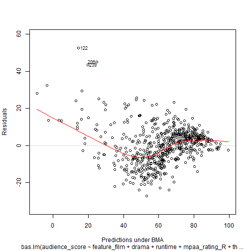
Figure 4.2 Model Probabilities
plot(bma_movies, which = 2, caption = "")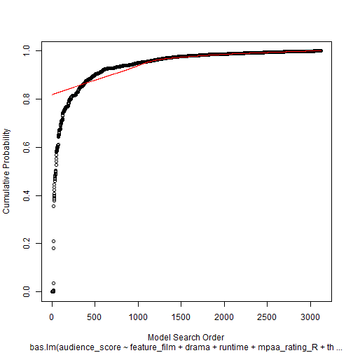
Figure 4.3 Model Complexity
plot(bma_movies, which = 3, caption = "", sub.caption = "")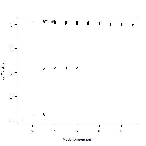
Figure 4.4 Inclusion Probabilities
plot(bma_movies, which = 4, caption = "", sub.caption = "")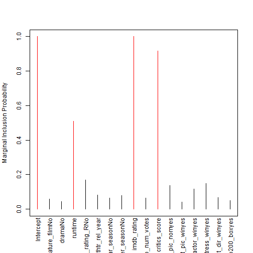
Figure 4.5 Model Rank
image(bma_movies, rotate = F)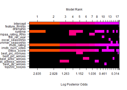
Part 5: Prediction
test_set <- movies_rm[,c(18,33,34,4,35,7,36,13,14,16,19,20,21,22,23,24,37)]


sausage_party <- data.frame(audience_score = 0, feature_film = "No", drama = "No", runtime = 89, mpaa_rating_R = "Yes",
                            thtr_rel_year = 2016, oscar_season = "No", imdb_rating = 7.5, imdb_num_votes = 3409, critics_score = 84,
                            best_pic_nom = "no", best_pic_win = "no", best_actor_win = "no", best_actress_win = "no", best_dir_win = "no", top200_box = "no", summer_season = "Yes")


new_set <- rbind(test_set, sausage_party)

BMA <- predict(bma_movies, newdata= new_set, top = 1, estimator = "BMA", prediction = TRUE, se.fit = TRUE)

predicted_value <- BMA$fit[620,]

ci_pred <- confint(BMA, estimator = "BMA")

ci_pred_value <- ci_pred[620,]

pred_table <- cbind(predicted_value, ci_pred_value)
Using the model build in section 4 of this report, I predicted the audience score for Sausage Party, a comedy released on August 12th. The predicted audience score for Sausage Party is 80.36 based on this model. The credible interval predicts that the the true audience score will be between 60.35 and 100.52 95% of the time. The prediction method uses a BMA process. To reiterate, there are three key factors that determine this prediction. The run time of the movie (1 hour and 29 minutes), the IMDB rating (7.5), and critics score from rotten tomateoes (84%).
Part 6: Conclusion
This report goes through the process of building a bayesian model to estimate audience scores for a movie given certian qualities. From a bayesian model averaging method the most important factors to include when predicting audience score are runtime, IMDB rating, and rotten tomatoes critics score. A larger sample of movies and reviews based on random selection would help provide causal interpretations to these coefficients. Future research could involve testing these optimal coefficicents in a more randomized and experimental fashion to examine their causal impact.