Description

Part of my job as a Data Scientist is calculating and analyzing test results. A big area of testing is around ad performance for different groups, creative types, or placements. By using the BayesianFirstAid package I can compare proportions and bring prio knowledge to the single test. This allows previous testing to play a part in future testing, and allows for results from smaller samples or shorter timelines. Below is an example of how the bayesian proportion test works from this package. A more detailed description can be found in the reference above.

Example

Lets say I have a test for two different placements running. They focus on the same demographic and randomly show Group 1 or Group 2 to each person in this demo. At the end of three weeks we have the conversions (or sales) and impressions served for each group. Group 1 has 20 conversions from 1,500 impressions and Group 2 has 45 conversions from 1,000 impressions. In this case our beta prio is uniform (0,0), but there are ways to adjust this prio if we have previous knowledge of the distribution of conversions. Now we compare these two groups using the bayes.prop.test() function.

library(devtools)
library(BayesianFirstAid)
 
conversions <- c(20,45)
impressions <- c(1500, 1000)
 
test <- bayes.prop.test(conversions, impressions)
test

 
 	Bayesian First Aid proportion test
 
 data: conversions out of impressions
 number of successes:    20,   45
 number of trials:     1500, 1000
 Estimated relative frequency of success [95% credible interval]:
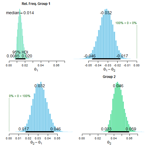
   Group 1: 0.014 [0.0084, 0.020]
   Group 2: 0.046 [0.033, 0.059]
 Estimated group difference (Group 1 - Group 2):
   -0.03 [-0.046, -0.018]
 The relative frequency of success is larger for Group 1 by a probability
 of <0.001 and larger for Group 2 by a probability of >0.999 .

The output shows the number of successes (conversions) and number of trials (impressions). Next the output provides the 95% credible interval for each group off of a MCMC simulation of 15,000 trials. This shows the conversion rate for each relative group. Next a simple subtraction of the difference in the credible intervals. Finally, an estimate of which group is larger.

The best way to examine group differneces is through a visual. By running a sample plot() call on the test we can examine the difference. The green distributuions are the 95% credible intervals for each group. The blue distributions are the differences between groups and the probability that the difference is zero (aka the groups are the same). In this case the two groups (which are different placements in our example) are drastically different. We now know with confidence that Group 2 performend much better, and whatever is different there should be how we optimize media.

Bayesian Proportion Test Visualization